val sua = Double.uniform()
val sub = Double.uniform(-1.0, 1.0)

val v2ua = Vector2.uniform()
val v2ub = Vector2.uniform(-1.0, 1.0)
val v2uc = Vector2.uniform(Vector2(0.0, 0.0), Vector2(1.0, 1.0))
val v2ur = Vector2.uniformRing(0.5, 1.0)

val v3ua = Vector3.uniform()
val v3ub = Vector3.uniform(-1.0, 1.0)
val v3uc = Vector3.uniform(Vector3(0.0, 0.0, 0.0), Vector3(1.0, 1.0, 1.0))
val v3ur = Vector3.uniformRing(0.5, 1.0)

val v4ua = Vector4.uniform()
val v4ub = Vector4.uniform(-1.0, 1.0)
val v4uc = Vector4.uniform(Vector4(0.0, 0.0, 0.0, 0.0), Vector4(1.0, 1.0, 1.0, 1.0))
val v4ur = Vector4.uniformRing(0.5, 1.0)

val ringSamples = List(500) { Vector2.uniformRing() }

Noise function composition

Since ORX 0.4 the orx-noise module comes with functional composition tooling that allow one to create complex noise functions.

// create an FBM version of 1D linear perlin noise
val myNoise0 = perlinLinear1D.fbm(octaves=3)
val noiseValue0 = myNoise0(431, seconds)

// create polar version of 2D simplex noise
val myNoise1 = simplex2D.withPolarInput()
val noiseValue1 = myNoise1(5509, Polar(seconds*60.0, 0.5))

// create value linear noise with squared outputs which is then billowed
val myNoise2 = valueLinear1D.mapOutput { it * it }.billow()
val noiseValue2 = myNoise2(993, seconds * 0.1)

Multi-dimensional noise

These are a mostly straight port from FastNoise-Java but have a slightly different interface.

Perlin noise

// -- 1d
val v0 = perlinLinear(seed, x)
val v1 = perlinQuintic(seed, x)
val v2 = perlinHermite(seed, x)

// -- 2d
val v3 = perlinLinear(seed, x, y)
val v4 = perlinQuintic(seed, x, y)
val v5 = perlinHermite(seed, x, y)

// -- 3d
val v6 = perlinLinear(seed, x, y, z)
val v7 = perlinQuintic(seed, x, y, z)
val v8 = perlinHermite(seed, x, y, z)

Value noise

// -- 1d
val v0 = valueLinear(seed, x)
val v1 = valueQuintic(seed, x)
val v2 = valueHermite(seed, x)

// -- 2d
val v2 = valueLinear(seed, x, y)
val v3 = valueQuintic(seed, x, y)
val v4 = valueHermite(seed, x, y)

// -- 3d
val v5 = valueLinear(seed, x, y, z)
val v6 = valueQuintic(seed, x, y, z)
val v7 = valueHermite(seed, x, y ,z)

Simplex noise

// -- 1d
val v0 = simplex(seed, x)

// -- 2d
val v1 = simplex(seed, x, y)

// -- 3d
val v2 = simplex(seed, x, y, z)

// -- 4d
val v3 = simplex(seed, x, y, z, w)

Cubic noise

// -- 1d
val v0 = cubic(seed, x, y)
val v1 = cubicQuintic(seed, x, y)
val v2 = cubicHermite(seed, x, y)

// -- 2d
val v0 = cubic(seed, x, y)
val v1 = cubicQuintic(seed, x, y)
val v2 = cubicHermite(seed, x, y)

// -- 3d
val v3 = cubic(seed, x, y, z)
val v4 = cubicQuintic(seed, x, y, z)
val v5 = cubicHermite(seed, x, y ,z)

Fractal noise

The library provides 3 functions with which fractal noise can be composed.

Fractal brownian motion (FBM)

// 1d
val v0 = fbm(seed, x, ::perlinLinear, octaves, lacunarity, gain)
val v1 = fbm(seed, x, ::simplex, octaves, lacunarity, gain)
val v2 = fbm(seed, x, ::valueLinear, octaves, lacunarity, gain)

// 2d
val v3 = fbm(seed, x, y, ::perlinLinear, octaves, lacunarity, gain)
val v4 = fbm(seed, x, y, ::simplex, octaves, lacunarity, gain)
val v5 = fbm(seed, x, y, ::valueLinear, octaves, lacunarity, gain)

// 3d
val v6 = fbm(seed, x, y, z, ::perlinLinear, octaves, lacunarity, gain)
val v7 = fbm(seed, x, y, z, ::simplex, octaves, lacunarity, gain)
val v8 = fbm(seed, x, y, z, ::valueLinear, octaves, lacunarity, gain)

Rigid

// 1d
val v0 = rigid(seed, x, ::perlinLinear, octaves, lacunarity, gain)
val v1 = rigid(seed, x, ::simplex, octaves, lacunarity, gain)
val v2 = rigid(seed, x, ::valueLinear, octaves, lacunarity, gain)

// 2d
val v2 = rigid(seed, x, y, ::perlinLinear, octaves, lacunarity, gain)
val v3 = rigid(seed, x, y, ::simplex, octaves, lacunarity, gain)
val v4 = rigid(seed, x, y, ::valueLinear, octaves, lacunarity, gain)

// 3d
val v3 = rigid(seed, x, y, z, ::perlinLinear, octaves, lacunarity, gain)
val v4 = rigid(seed, x, y, z, ::simplex, octaves, lacunarity, gain)
val v5 = rigid(seed, x, y, z, ::valueLinear, octaves, lacunarity, gain)

Billow

// 1d
val v0 = billow(seed, x, ::perlinLinear, octaves, lacunarity, gain)
val v1 = billow(seed, x, ::perlinLinear, octaves, lacunarity, gain)
val v2 = billow(seed, x, ::perlinLinear, octaves, lacunarity, gain)

// 2d
val v3 = billow(seed, x, y, ::perlinLinear, octaves, lacunarity, gain)
val v4 = billow(seed, x, y, ::perlinLinear, octaves, lacunarity, gain)
val v5 = billow(seed, x, y, ::perlinLinear, octaves, lacunarity, gain)

// 3d
val v6 = billow(seed, x, y, z, ::perlinLinear, octaves, lacunarity, gain)
val v7 = billow(seed, x, y, z, ::perlinLinear, octaves, lacunarity, gain)
val v8 = billow(seed, x, y, z, ::perlinLinear, octaves, lacunarity, gain)

Demos

DemoBla

source code

DemoCubicNoise2D01

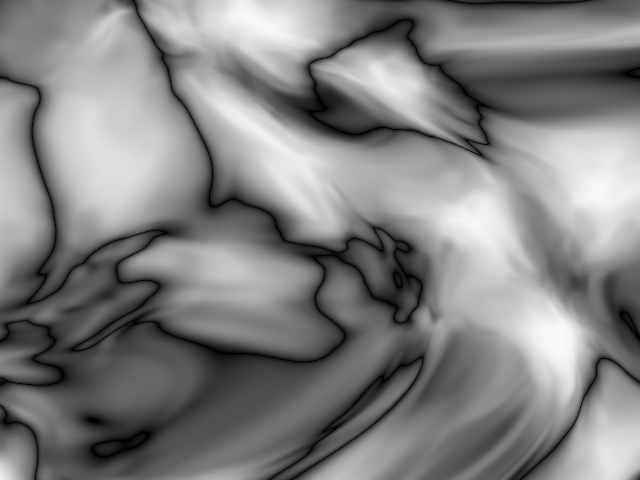
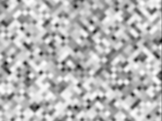
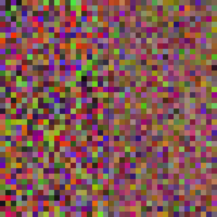
Demonstrates how to render dynamic grayscale patterns using 3D cubic Hermite interpolation. The program draws one point per pixel on the screen, calculating the color intensity of each point based on a 3D cubic Hermite noise function.

source code

DemoFunctionalComposition01

Demonstrates how to chain methods behind noise functions like simplex3D to alter its output. By default simplex3D produces one double value, but by calling .withVector2Output() it produces Vector2 instances instead.

The .gradient() method alters the output to return the direction of fastest increase. Read more in WikiPedia.

source code

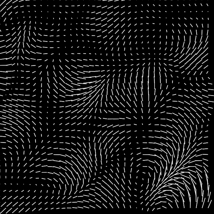
DemoGradientPerturb2D

Demonstrates how to generate a dynamic fractal-based visual effect using 2D gradient perturbation and simplex noise.

This method initializes a color buffer to create an image and applies fractal gradient noise to set each pixel's brightness, producing a dynamic visual texture. The fractal effect is achieved by layering multiple levels of noise, and each pixel's color intensity is based on the noise function results. The output is continuously updated to produce animated patterns.

CPU-based.

source code

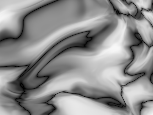
DemoGradientPerturb3D

Demonstrates how to generate a dynamically evolving visual representation of fractal noise. The program uses 3D gradient perturbation and simplex noise to produce a grayscale gradient on a color buffer.

The visual output is created by iteratively computing the fractal gradient perturbation and simplex noise for each pixel in the color buffer, applying a perturbation based on time, and rendering the result as an image.

CPU-based.

source code

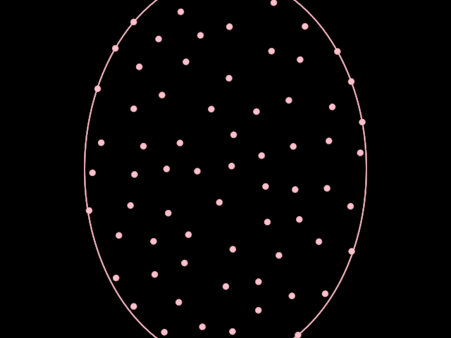
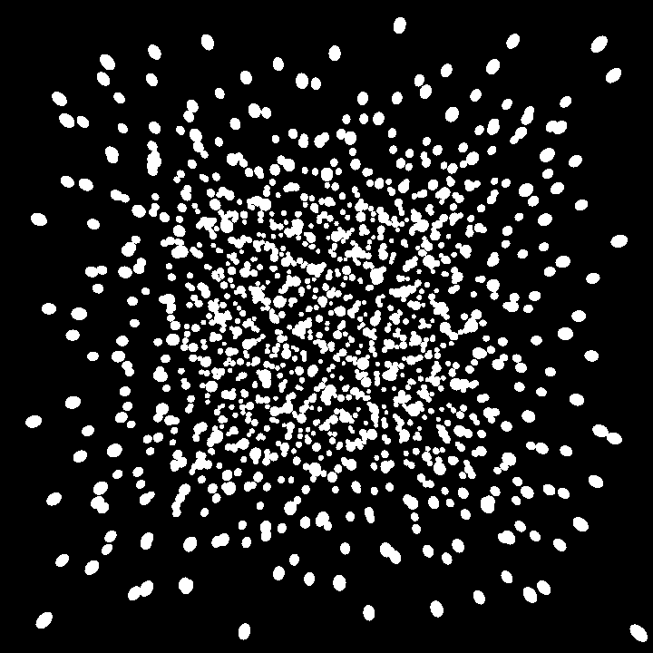
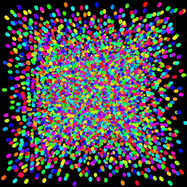
DemoScatter01

Demonstrates how to create an animated visualization of scattered points.

The program creates an animated ellipse with increasing and decreasing height. Then, scatters points inside it with a placementRadius of 20.0.

The animation reveals that the scattering positions are somewhat stable between animation frames.

The ellipse's contour is revealed and hidden every other second.

source code

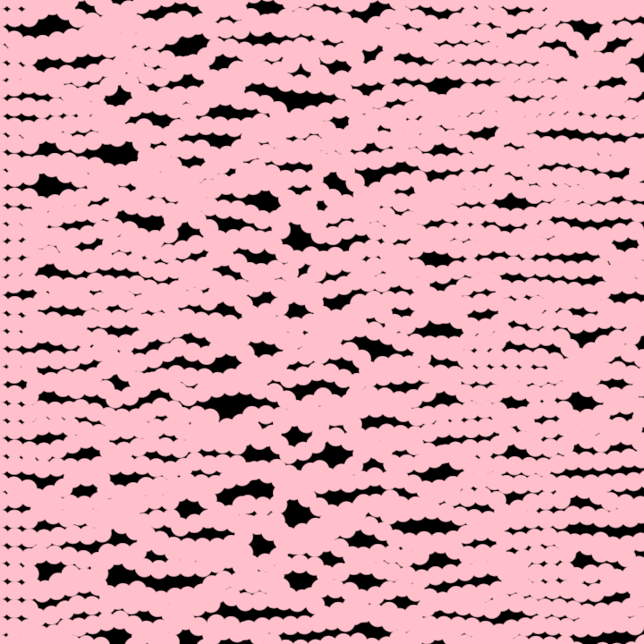
DemoSimplex01

Demonstrates how to use the simplex method to obtain noise values based on a seed and an x value.

The program creates 20 horizontal contours with 40 steps each in which each 2D step and each 2D control point is affected by noise.

Time is used as a noise argument to produce an animated effect.

source code

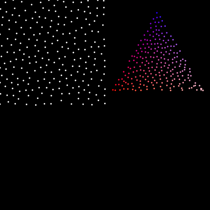
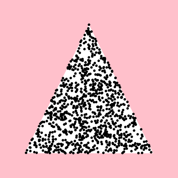
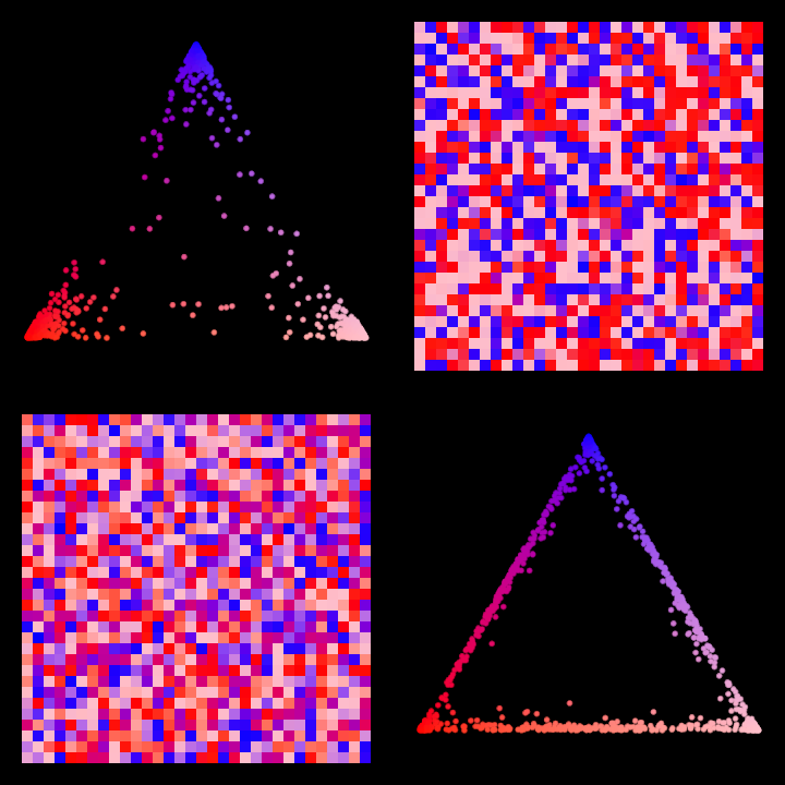
DemoTriangleNoise01

Demonstrate the generation of uniformly distributed points inside a list of triangles. For demonstration purposes there is only one triangle in the list, but could contain many.

We can consider the hash function as giving us access to a slice in a pool of random Vector2 values. Since we increase the x argument in the call to hash() based on the current time in seconds, older random points get replaced by newer ones, then stay visible for a while.

source code

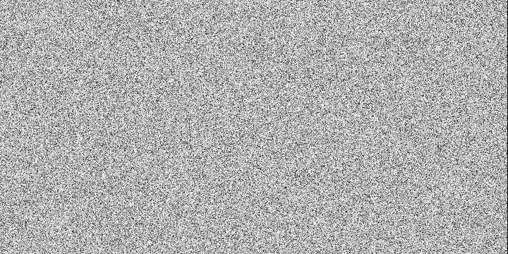
DemoValueNoise2D01

Demonstrates how to render grayscale noise patterns dynamically using 3D quintic noise.

The program draws one point per pixel on the screen, calculating the color intensity of each point based on a 3D quintic noise function. The noise value is influenced by the pixel's 2D coordinates and animated over time.

source code

glsl/DemoNoisesGLSLGui

Render existing GLSL noise algorithms side by side. Use the GUI to explore the effects.

source code

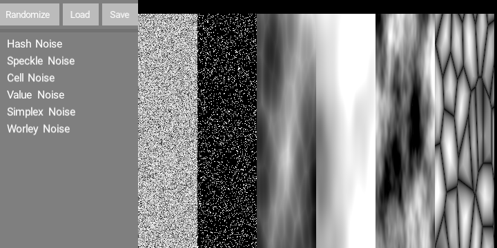
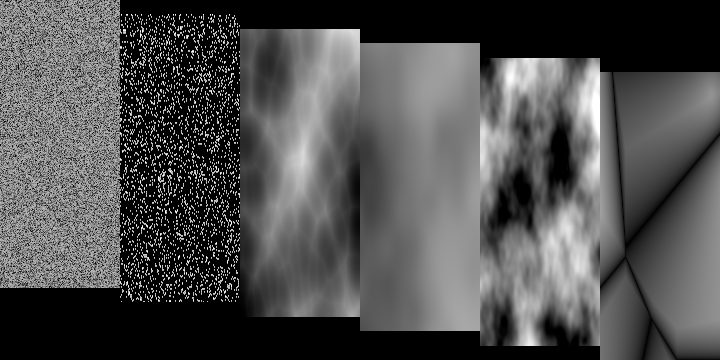
glsl/DemoNoisesGLSL

Render existing GLSL noise algorithms side by side. Re-use the same color buffer for the rendering. Not all noise properties are used. Explore each noise class to find out more adjustable properties. The noise color can be set using a color or a gain property.

source code

glsl/DemoSimplexGLSL

Render an animated Simplex3D texture using shaders.

The uniforms in the shader are controlled by randomized sine oscillators.

source code

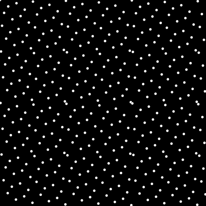
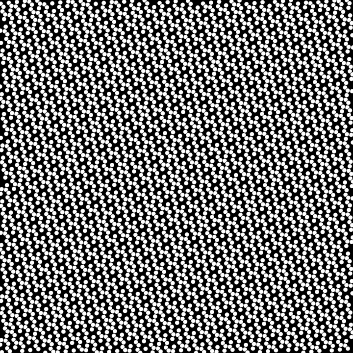
hammersley/DemoHammersley2D01

Demo that visualizes a 2D Hammersley point set.

The program computes 400 2D Hammersley points mapped within the window bounds. These points are visualized by rendering circles at their respective positions.

source code

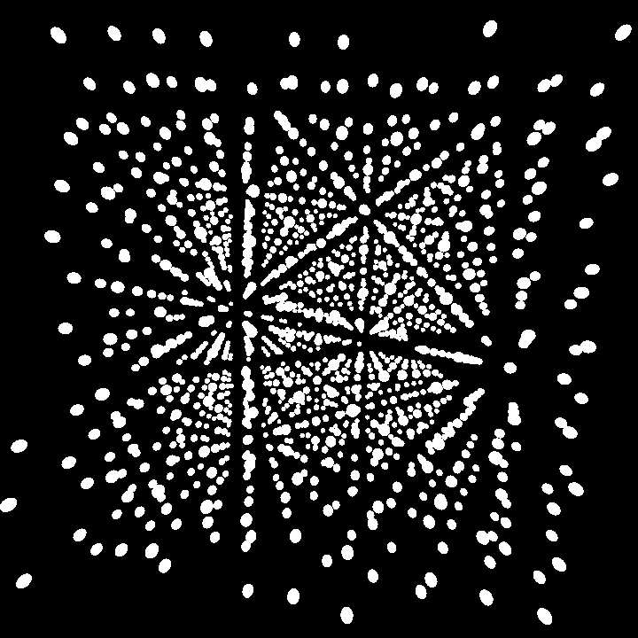
hammersley/DemoHammersley3D01

Demo program rendering a 3D visualization of points distributed using the Hammersley sequence in 3D space.

A set of 1400 points is generated using the Hammersley sequence. Each point is translated and rendered as a small sphere in 3D space.

The rendering uses the Orbital extension, enabling an interactive 3D camera to navigate the scene.

source code

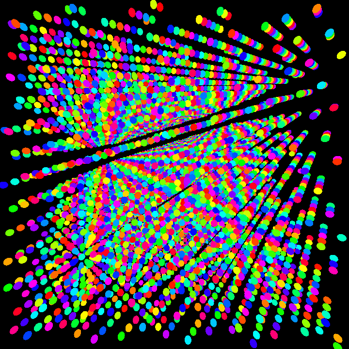
hammersley/DemoHammersley4D01

Demo visualizing a 4D Hammersley point set in a 3D space, with colors determined by the 4th dimension.

A total of 10,000 4D points are generated with the hammersley4D sequence. These points are mapped to a cubical volume and rendered as small spheres. The color of each sphere is modified based on the 4th dimension of its corresponding point by shifting the hue in HSV color space.

This program employs the Orbital extension, enabling camera interaction for 3D navigation of the scene.

source code

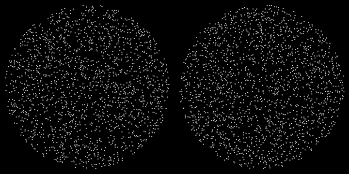
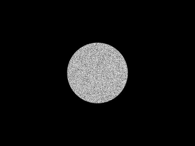
hash/DemoCircleHash01

Demonstrates how to draw circles distributed within two subregions of a rectangular area using uniform random distribution and a hash-based method for randomness.

The application divides the window area into two subregions, offsets the edges inwards, and then calculates two circles representing these subregions. Points are then generated and drawn within these circles using two different methods:

A uniform random distribution within the first circle.
A hash-based deterministic random point generation within the second circle.

source code

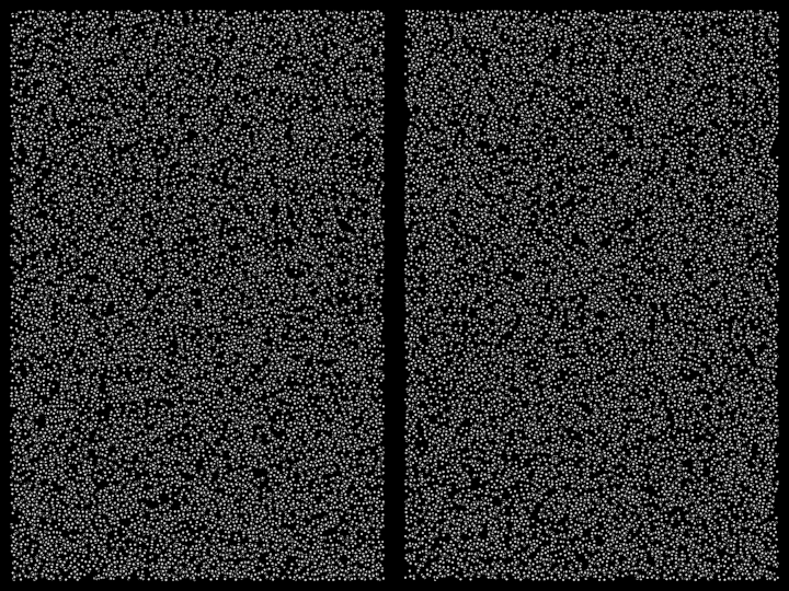
hash/DemoRectangleHash01

Demonstrates how to generate and draw random points within two subregions of a rectangular area using two different randomization methods.

The first subregion generates points using a uniform random distribution, while the second subregion generates points deterministically with a hash-based randomization approach. The points are visualized as small circles.

source code

hash/DemoUHash01

Demonstrates how to render a dynamic grid of points where the color of each point is determined using a hash-based noise generation method.

The application dynamically updates the visual output by calculating a 3D hash value for each point in the grid, based on the current time and the point's coordinates. The hash value is then used to determine the grayscale color intensity of each point.

source code

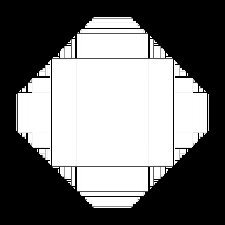
linearrange/DemoLinearRange01

Demonstrates how to create a linear range with two [org.openrndr.shape.Rectangle]s.

This range is then sampled at 100 random locations using the uniform method to get and render interpolated rectangles. The random seed changes once per second.

source code

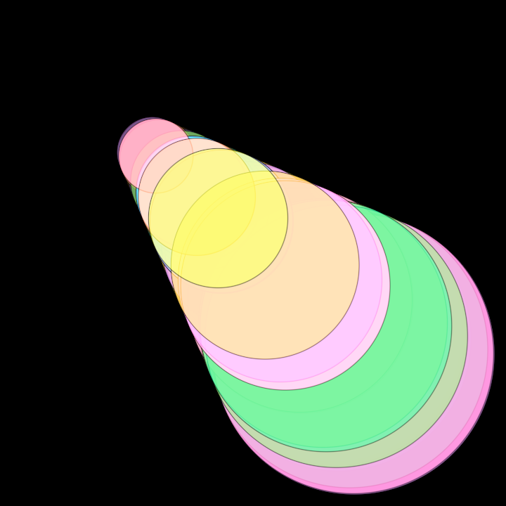
linearrange/DemoLinearRange02

Demonstrates how to create a linear range with two [org.openrndr.shape.Circle]s.

This range is then sampled at 100 random locations using the hash method to get and render interpolated circles. The random seed changes once per second.

Colors are calculated based on the index of each circle.

source code

phrases/DemoUHashPhrase01

Demonstrate the use of a uniform hashing function phrase in a ShadeStyle.

The hashing function uses the screen coordinates and the current time to calculate the brightness of each pixel.

Multiple GLSL hashing functions are defined in orx-shader-phrases.

source code

rseq/DemoRseq2D01

Demonstrates quasirandomly distributed 2D points. The points are generated using the R2 sequence and drawn as circles with a radius of 5.0.

source code

rseq/DemoRseq3D01

This demo renders a 3D visualization of points distributed using the R3 quasirandom sequence. Each point is represented as a sphere and positioned in 3D space based on the quasirandom sequence values.

The visualization setup includes:

Usage of an orbital camera for interactive 3D navigation.
Creation of a reusable sphere mesh with a specified radius.
Generation of quasirandom points in 3D space using the rSeq3D function.
Transformation and rendering of each point as a sphere using vertex buffers.

source code

rseq/DemoRseq4D01

Demo that presents a 3D visualization of points distributed using a 4D quasirandom sequence (R4). Each point is represented as a sphere with its position and color derived from the sequence values.

This function performs the following tasks:

Initializes a 3D camera for orbital navigation of the scene.
Generates 10,000 points in 4D space using the rSeq4D function. The points are scaled and transformed into 3D positions with an additional w-coordinate for color variation.
Creates a reusable sphere mesh for rendering.
Renders each point as a sphere with its position determined by the 3D coordinates of the point and its color calculated by shifting the hue of a base color using the w-coordinate value.

source code

simplexrange/DemoSimplexRange2D01

This demo creates a dynamic graphical output utilizing simplex and linear interpolation-based color ranges.

Functionalities:

Defines a list of base colors converted to LAB color space for smooth interpolation.
Constructs a 3D simplex range and a 2D linear range for color sampling.
Randomly populates two sections of the screen with rectangles filled with colors sampled from simplex and linear ranges respectively.
Draws a vertical divider line in the middle of the application window.

source code

simplexrange/DemoSimplexRange2D02

This demo creates a dynamic graphical output utilizing simplex and linear interpolation-based color ranges.

Functionalities:

Defines a list of base colors converted to LAB color space for smooth interpolation.
Constructs a 3D simplex range and a 2D linear range for color sampling.
Randomly populates two sections of the screen with rectangles filled with colors sampled from simplex and linear ranges respectively.
Draws a vertical divider line in the middle of the application window.

source code

simplexrange/DemoSimplexUniform01

This demo creates a dynamic graphical output utilizing simplex and linear interpolation-based color ranges.

Functionalities:

Defines a list of base colors converted to LAB color space for smooth interpolation.
Constructs a 3D simplex range and a 2D linear range for color sampling.
Randomly populates two sections of the screen with rectangles filled with colors sampled from simplex and linear ranges respectively.
Draws a vertical divider line in the middle of the application window.

source code

simplexrange/DemoSimplexUniform02

This demo creates a dynamic graphical output utilizing simplex and linear interpolation-based color ranges.

Functionalities:

Defines a list of base colors converted to LAB color space for smooth interpolation.
Constructs a 3D simplex range and a 2D linear range for color sampling.
Randomly populates two sections of the screen with rectangles filled with colors sampled from simplex and linear ranges respectively.
Draws a vertical divider line in the middle of the application window.

source code