orx/orx-noise

orx-noise

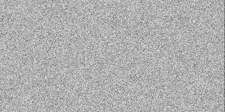
Randomness for every type of person: Perlin, uniform, value, simplex, fractal and many other types of noise.

Uniform random numbers

val sua = Double.uniform()
val sub = Double.uniform(-1.0, 1.0)

val v2ua = Vector2.uniform()
val v2ub = Vector2.uniform(-1.0, 1.0)
val v2uc = Vector2.uniform(Vector2(0.0, 0.0), Vector2(1.0, 1.0))
val v2ur = Vector2.uniformRing(0.5, 1.0)

val v3ua = Vector3.uniform()
val v3ub = Vector3.uniform(-1.0, 1.0)
val v3uc = Vector3.uniform(Vector3(0.0, 0.0, 0.0), Vector3(1.0, 1.0, 1.0))
val v3ur = Vector3.uniformRing(0.5, 1.0)

val v4ua = Vector4.uniform()
val v4ub = Vector4.uniform(-1.0, 1.0)
val v4uc = Vector4.uniform(Vector4(0.0, 0.0, 0.0, 0.0), Vector4(1.0, 1.0, 1.0, 1.0))
val v4ur = Vector4.uniformRing(0.5, 1.0)

val ringSamples = List(500) { Vector2.uniformRing() }

Noise function composition

Since ORX 0.4 the orx-noise module comes with functional composition tooling that allow one to create complex noise functions.

// create an FBM version of 1D linear perlin noise
val myNoise0 = perlinLinear1D.fbm(octaves=3)
val noiseValue0 = myNoise0(431, seconds)

// create polar version of 2D simplex noise
val myNoise1 = simplex2D.withPolarInput()
val noiseValue1 = myNoise1(5509, Polar(seconds*60.0, 0.5))

// create value linear noise with squared outputs which is then billowed
val myNoise2 = valueLinear1D.mapOutput { it * it }.billow()
val noiseValue2 = myNoise2(993, seconds * 0.1)

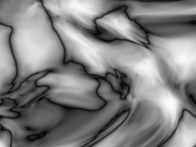
Multi-dimensional noise

These are a mostly straight port from FastNoise-Java but have a slightly different interface.

Perlin noise

// -- 1d
val v0 = perlinLinear(seed, x)
val v1 = perlinQuintic(seed, x)
val v2 = perlinHermite(seed, x)

// -- 2d
val v3 = perlinLinear(seed, x, y)
val v4 = perlinQuintic(seed, x, y)
val v5 = perlinHermite(seed, x, y)

// -- 3d
val v6 = perlinLinear(seed, x, y, z)
val v7 = perlinQuintic(seed, x, y, z)
val v8 = perlinHermite(seed, x, y, z)

Value noise

// -- 1d
val v0 = valueLinear(seed, x)
val v1 = valueQuintic(seed, x)
val v2 = valueHermite(seed, x)

// -- 2d
val v2 = valueLinear(seed, x, y)
val v3 = valueQuintic(seed, x, y)
val v4 = valueHermite(seed, x, y)

// -- 3d
val v5 = valueLinear(seed, x, y, z)
val v6 = valueQuintic(seed, x, y, z)
val v7 = valueHermite(seed, x, y ,z)

Simplex noise

// -- 1d
val v0 = simplex(seed, x)

// -- 2d
val v1 = simplex(seed, x, y)

// -- 3d
val v2 = simplex(seed, x, y, z)

// -- 4d
val v3 = simplex(seed, x, y, z, w)

Cubic noise

// -- 1d
val v0 = cubic(seed, x, y)
val v1 = cubicQuintic(seed, x, y)
val v2 = cubicHermite(seed, x, y)

// -- 2d
val v0 = cubic(seed, x, y)
val v1 = cubicQuintic(seed, x, y)
val v2 = cubicHermite(seed, x, y)

// -- 3d
val v3 = cubic(seed, x, y, z)
val v4 = cubicQuintic(seed, x, y, z)
val v5 = cubicHermite(seed, x, y ,z)

Fractal noise

The library provides 3 functions with which fractal noise can be composed.

Fractal brownian motion (FBM)

// 1d
val v0 = fbm(seed, x, ::perlinLinear, octaves, lacunarity, gain)
val v1 = fbm(seed, x, ::simplex, octaves, lacunarity, gain)
val v2 = fbm(seed, x, ::valueLinear, octaves, lacunarity, gain)

// 2d
val v3 = fbm(seed, x, y, ::perlinLinear, octaves, lacunarity, gain)
val v4 = fbm(seed, x, y, ::simplex, octaves, lacunarity, gain)
val v5 = fbm(seed, x, y, ::valueLinear, octaves, lacunarity, gain)

// 3d
val v6 = fbm(seed, x, y, z, ::perlinLinear, octaves, lacunarity, gain)
val v7 = fbm(seed, x, y, z, ::simplex, octaves, lacunarity, gain)
val v8 = fbm(seed, x, y, z, ::valueLinear, octaves, lacunarity, gain)

Rigid

// 1d
val v0 = rigid(seed, x, ::perlinLinear, octaves, lacunarity, gain)
val v1 = rigid(seed, x, ::simplex, octaves, lacunarity, gain)
val v2 = rigid(seed, x, ::valueLinear, octaves, lacunarity, gain)

// 2d
val v2 = rigid(seed, x, y, ::perlinLinear, octaves, lacunarity, gain)
val v3 = rigid(seed, x, y, ::simplex, octaves, lacunarity, gain)
val v4 = rigid(seed, x, y, ::valueLinear, octaves, lacunarity, gain)

// 3d
val v3 = rigid(seed, x, y, z, ::perlinLinear, octaves, lacunarity, gain)
val v4 = rigid(seed, x, y, z, ::simplex, octaves, lacunarity, gain)
val v5 = rigid(seed, x, y, z, ::valueLinear, octaves, lacunarity, gain)

Billow

// 1d
val v0 = billow(seed, x, ::perlinLinear, octaves, lacunarity, gain)
val v1 = billow(seed, x, ::perlinLinear, octaves, lacunarity, gain)
val v2 = billow(seed, x, ::perlinLinear, octaves, lacunarity, gain)

// 2d
val v3 = billow(seed, x, y, ::perlinLinear, octaves, lacunarity, gain)
val v4 = billow(seed, x, y, ::perlinLinear, octaves, lacunarity, gain)
val v5 = billow(seed, x, y, ::perlinLinear, octaves, lacunarity, gain)

// 3d
val v6 = billow(seed, x, y, z, ::perlinLinear, octaves, lacunarity, gain)
val v7 = billow(seed, x, y, z, ::perlinLinear, octaves, lacunarity, gain)
val v8 = billow(seed, x, y, z, ::perlinLinear, octaves, lacunarity, gain)

Demos

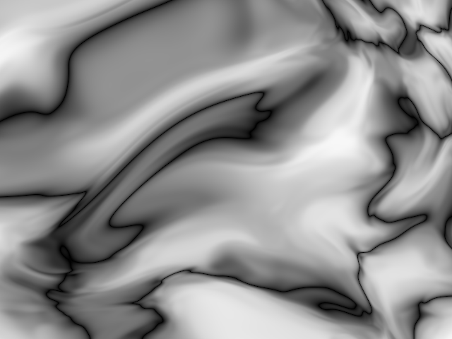
DemoCubicNoise2D01

source code

DemoFunctionalComposition01

source code

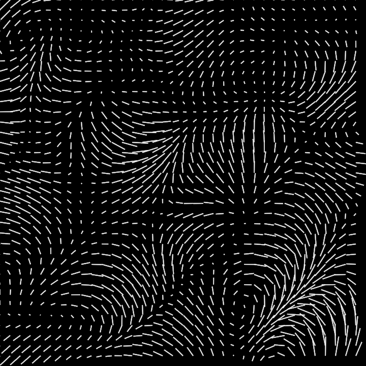
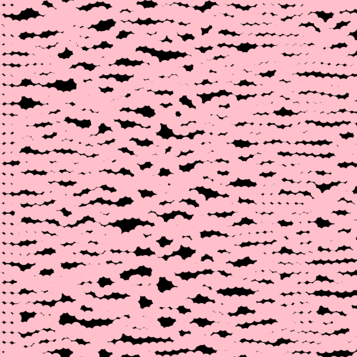
DemoGradientPerturb2D

source code

DemoGradientPerturb3D

source code

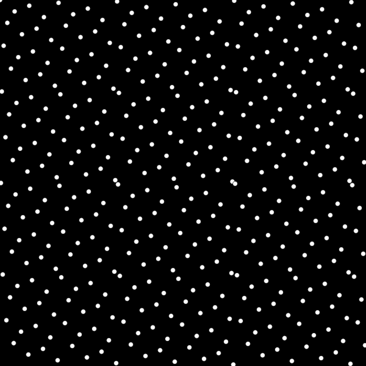
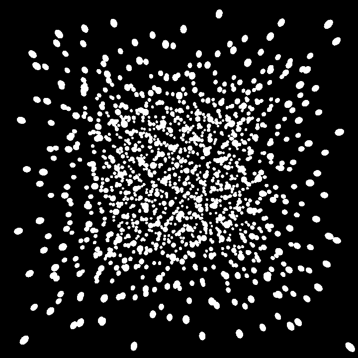
DemoScatter01

source code

DemoSimplex01

source code

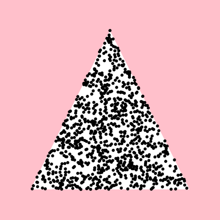
DemoTriangleNoise01

Demonstrate the generation of uniformly distributed points inside a list of triangles

source code

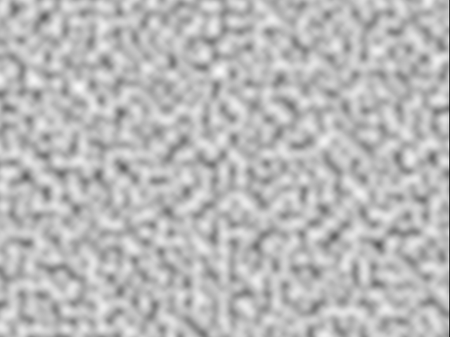
DemoValueNoise2D01

source code

glsl/DemoNoisesGLSLGui

Render existing GLSL noise algorithms side by side. Use the GUI to explore the effects.

source code

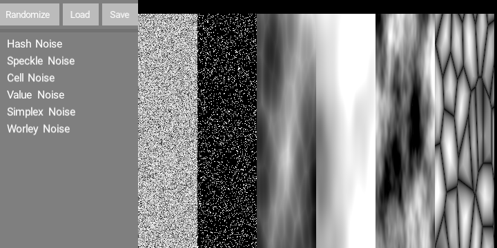
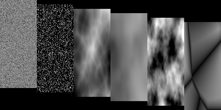
glsl/DemoNoisesGLSL

Render existing GLSL noise algorithms side by side. Re-use the same color buffer for the rendering. Not all noise properties are used. Explore each noise class to find out more adjustable properties. The noise color can be set using a color or a gain property.

source code

glsl/DemoSimplexGLSL

A sine oscillator with randomized parameters

source code

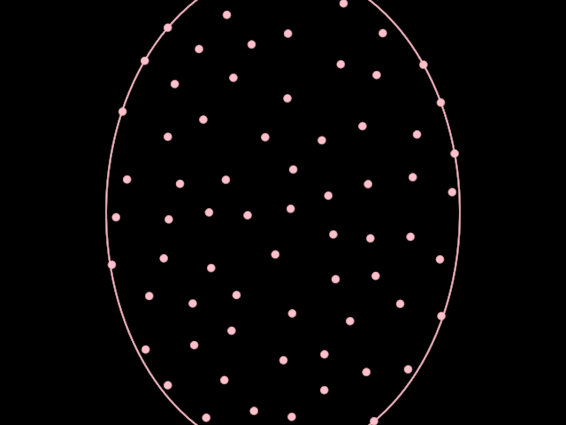
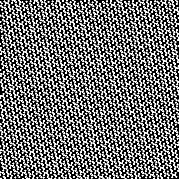
hammersley/DemoHammersley2D01

Demo that visualizes a 2D Hammersley point set.

The application is configured to run at 720x720 resolution. The program computes 400 2D Hammersley points mapped within the bounds of the application's resolution. These points are visualized by rendering circles at their respective positions.

source code

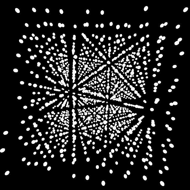
hammersley/DemoHammersley3D01

Demo program rendering a 3D visualization of points distributed using the Hammersley sequence in 3D space.

The application is set up at a resolution of 720x720 pixels. Within the visual program, a sphere mesh is created and a set of 1400 points is generated using the Hammersley sequence. Each point is translated and rendered as a small sphere in 3D space. This is achieved by mapping the generated points into a scaled domain.

The rendering utilizes the Orbital extension, enabling an interactive 3D camera to navigate the scene. The visualization relies on the draw loop for continuous rendering of the points.

source code

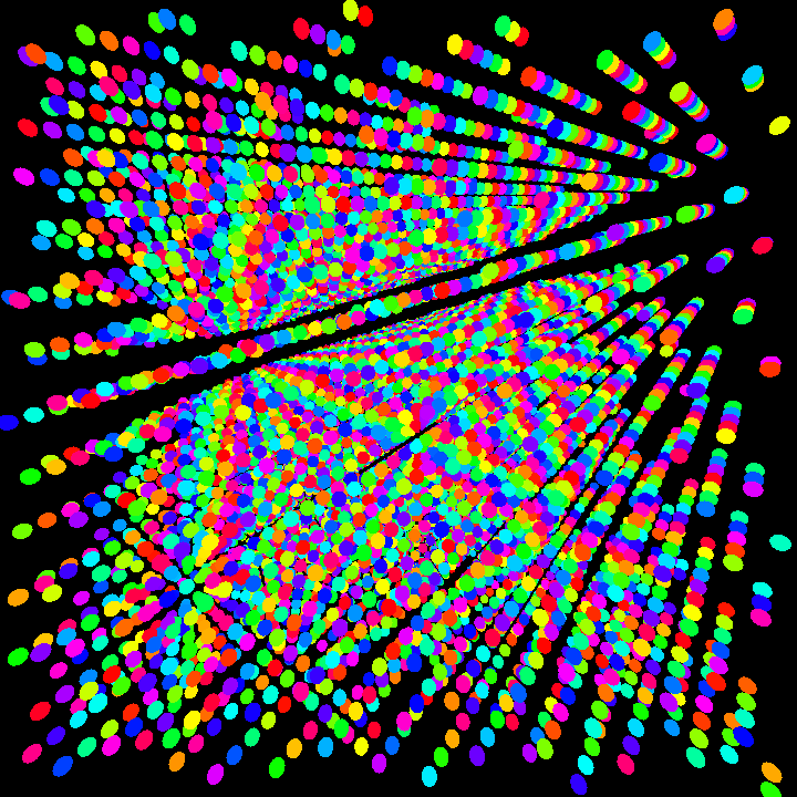
hammersley/DemoHammersley4D01

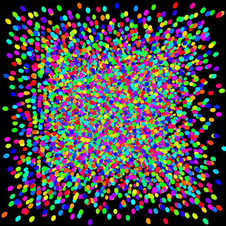
Demo that visualizes a 4D Hammersley point set in a 3D space, with colors determined by the 4th dimension.

The application is configured at a resolution of 720x720 pixels. A sphere mesh is created using the sphereMesh utility, and a total of 10,000 4D points are generated with the hammersley4D sequence. These points are scaled, translated, and rendered as small spheres. The color of each sphere is modified based on the 4th dimension of its corresponding point by shifting the hue in HSV color space.

This program employs the Orbital extension, enabling camera interaction for 3D navigation of the scene. Rendering occurs within the draw loop, providing continuous visualization of the point distribution.

source code

hash/DemoCircleHash01

source code

hash/DemoRectangleHash01

source code

hash/DemoUHash01

source code

linearrange/DemoLinearRange01

source code

phrases/DemoUHashPhrase01

Demonstrate uniform hashing function phrase in a shadestyle

source code

rseq/DemoRseq2D01

This demo sets up a window with dimensions 720x720 and renders frames demonstrating 2D quasirandomly distributed points. The points are generated using the R2 sequence and drawn as circles with a radius of 5.0.

source code

rseq/DemoRseq3D01

This demo renders a 3D visualizationof points distributed using the R3 quasirandom sequence. Each point is represented as a sphere and positioned in 3D space based on the quasirandom sequence values.

The visualization setup includes:

• Configuration of application window size to 720x720.
• Usage of an orbital camera for interactive 3D navigation.
• Creation of a reusable sphere mesh with a specified radius.
• Generation of quasirandom points in 3D space using the rSeq3D function.
• Transformation and rendering of each point as a sphere using vertex buffers.

source code

rseq/DemoRseq4D01

Demo that presents a 3D visualization of points distributed using a 4D quasirandom sequence (R4). Each point is represented as a sphere with it position and color derived from the sequence values.

This function performs the following tasks:

• Configures the application window dimensions to 720x720 pixels.
• Initializes a 3D camera for orbital navigation of the scene.
• Generates 10,000 points in 4D space using the rSeq4D function. The points are scaled and transformed into 3D positions with an additional w-coordinate for color variation.
• Creates a reusable sphere mesh for rendering.
• Renders each point as a sphere with its position determined by the 3D coordinates of the point and its color calculated by shifting the hue of a base color using the w-coordinate value.

source code

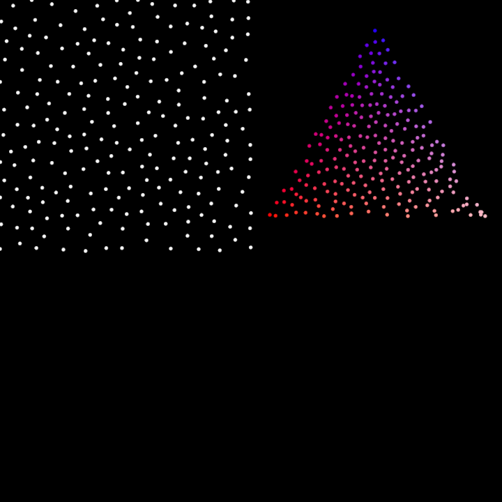
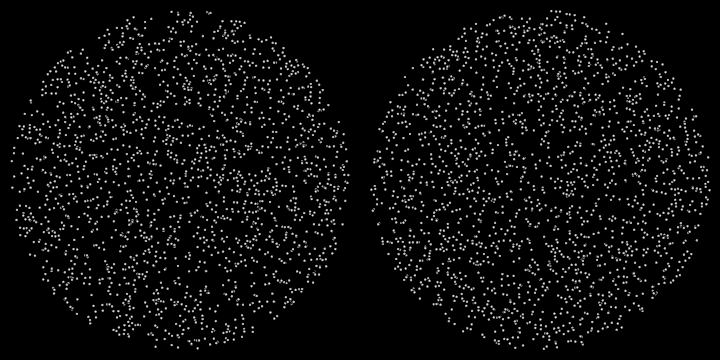
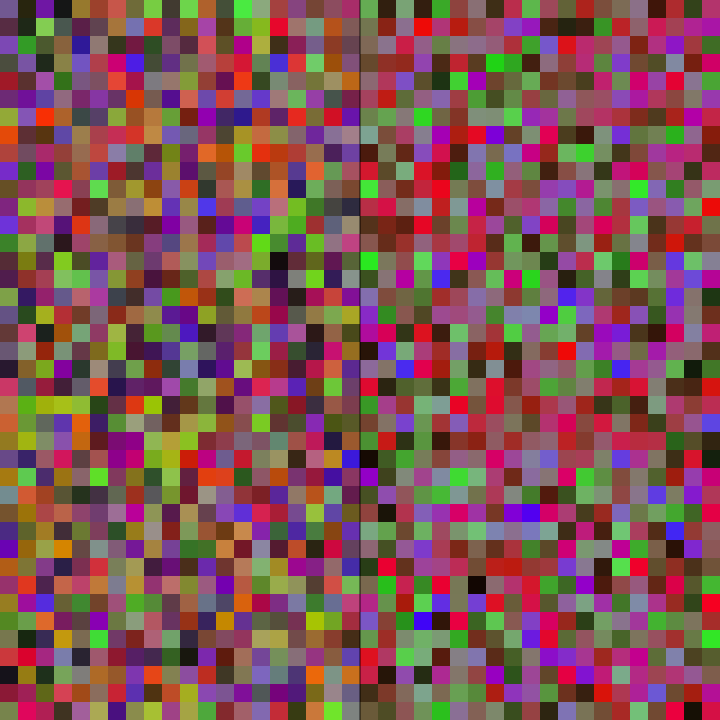
simplexrange/DemoSimplexRange2D01

This demo creates a dynamic graphical output utilizing simplex and linear interpolation-based color ranges.

Functionalities:

• Defines a list of base colors converted to LAB color space for smooth interpolation.
• Constructs a 3D simplex range and a 2D linear range for color sampling.
• Randomly populates two sections of the screen with rectangles filled with colors sampled from simplex and linear ranges respectively.
• Draws a vertical divider line in the middle of the application window.

source code

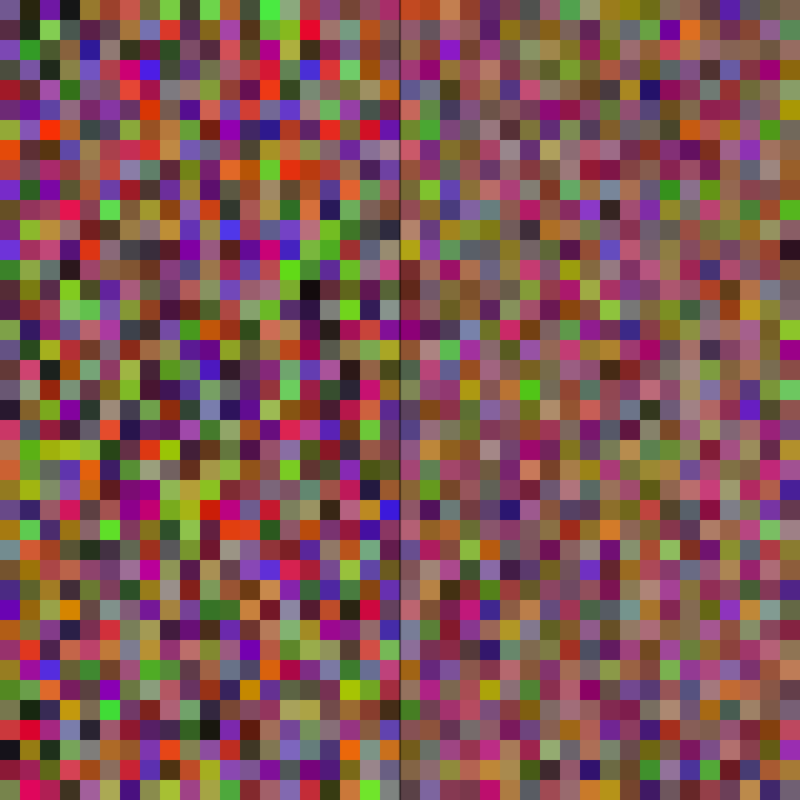
simplexrange/DemoSimplexRange2D02

This demo creates a dynamic graphical output utilizing simplex and linear interpolation-based color ranges.

Functionalities:

• Defines a list of base colors converted to LAB color space for smooth interpolation.
• Constructs a 3D simplex range and a 2D linear range for color sampling.
• Randomly populates two sections of the screen with rectangles filled with colors sampled from simplex and linear ranges respectively.
• Draws a vertical divider line in the middle of the application window.

source code

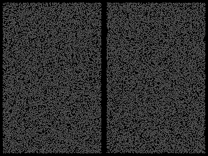
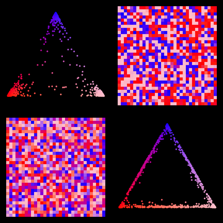
simplexrange/DemoSimplexUniform01

This demo creates a dynamic graphical output utilizing simplex and linear interpolation-based color ranges.

Functionalities:

• Defines a list of base colors converted to LAB color space for smooth interpolation.
• Constructs a 3D simplex range and a 2D linear range for color sampling.
• Randomly populates two sections of the screen with rectangles filled with colors sampled from simplex and linear ranges respectively.
• Draws a vertical divider line in the middle of the application window.

source code

simplexrange/DemoSimplexUniform02

This demo creates a dynamic graphical output utilizing simplex and linear interpolation-based color ranges.

Functionalities:

• Defines a list of base colors converted to LAB color space for smooth interpolation.
• Constructs a 3D simplex range and a 2D linear range for color sampling.
• Randomly populates two sections of the screen with rectangles filled with colors sampled from simplex and linear ranges respectively.
• Draws a vertical divider line in the middle of the application window.

source code