orx/orx-math/README.md

orx-math

Mathematical utilities, including complex numbers, linear ranges, simplex ranges, matrices and radial basis functions (RBF).

Demos

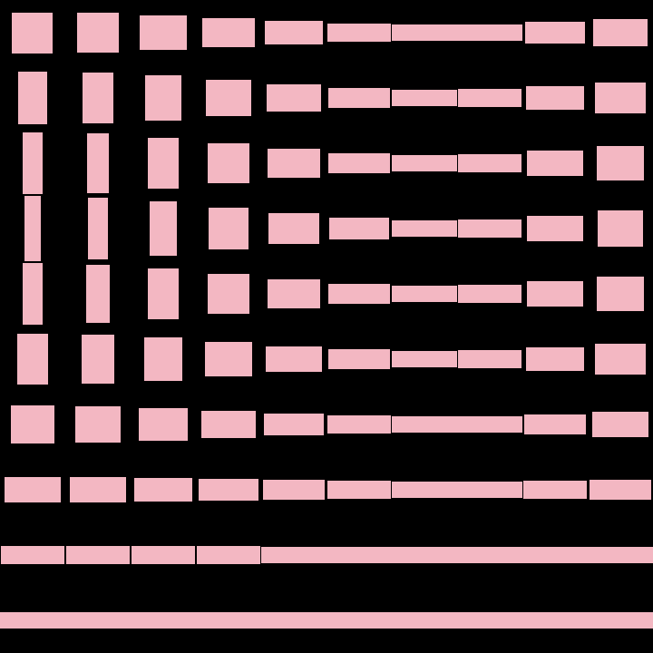
linearrange/DemoLinearRange02

Demonstrate how to create a 1D linear range between two instances of a LinearType, in this case, a horizontal Rectangle and a vertical one.

Notice how the .. operator is used to construct the LinearRange1D.

The resulting LinearRange1D provides a value() method that takes a normalized input and returns an interpolated value between the two input elements.

This example draws a grid of rectangles interpolated between the horizontal and the vertical triangles. The x and y coordinates and the seconds variable are used to specify the interpolation value for each grid cell.

One can use the LinearRange class to construct

• a LinearRange2D out of two LinearRange1D
• a LinearRange3D out of two LinearRange2D
• a LinearRange4D out of two LinearRange3D

(not demonstrated here)

source code

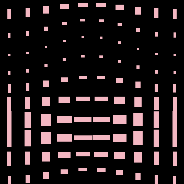
linearrange/DemoLinearRange03

Demonstrates how to create a LinearRange2D out of two LinearRange1D instances. The first range interpolates a horizontal rectangle into a vertical one. The second range interpolates two smaller squares of equal size, one placed higher along the y-axis and another one lower.

A grid of such rectangles is displayed, animating the u and v parameters based on seconds, x and y indices. The second range results in a vertical wave effect.

source code

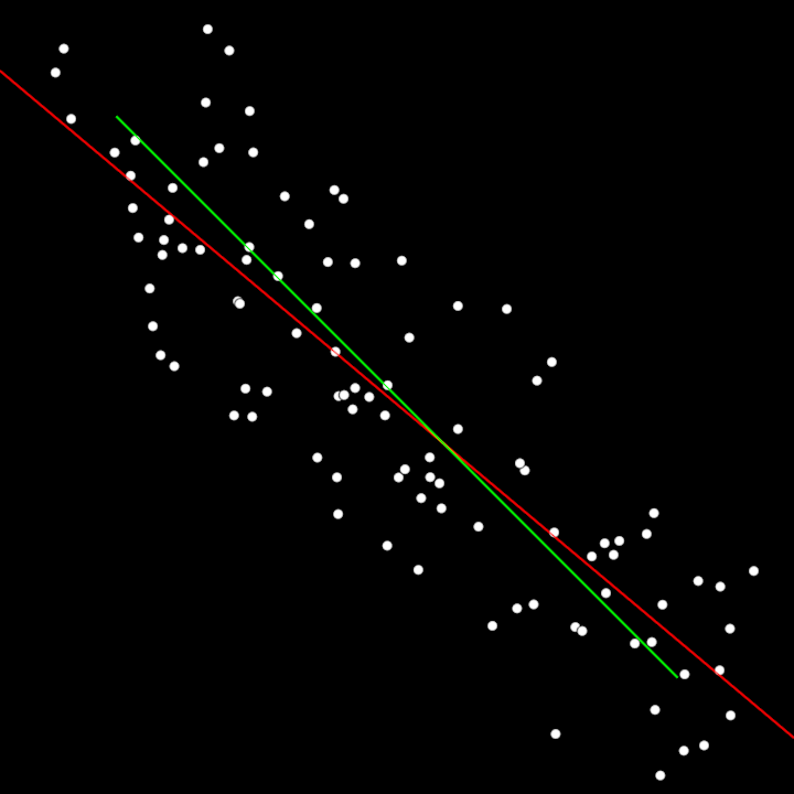
matrix/DemoLeastSquares01

Demonstrate least squares method to find a regression line through noisy points. The line drawn in red is the estimated line. The green one is the ground-truth.

Ax = b => x = A⁻¹b because A is likely inconsistent, we look for an approximate x based on AᵀA, which is consistent. x̂ = (AᵀA)⁻¹ Aᵀb

source code

matrix/DemoLeastSquares02

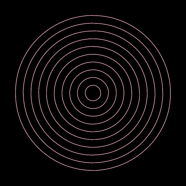
Demonstrate how to use the least squares method to fit a cubic bezier to noisy points.

On every animation frame, 10 concentric circles are created centered on the window and converted to contours. In OPENRNDR, circular contours are made ouf of 4 cubic-Bezier curves. Each of those curves is considered one by one as the ground truth, then 5 points are sampled near those curves. Finally, two matrices are constructed using those points and math operations are applied to revert the randomization attempting to reconstruct the original curves.

The result is drawn on every animation frame, revealing concentric circles that are more or less similar to the ground truth depending on the random values used.

source code

rbf/RbfInterpolation01

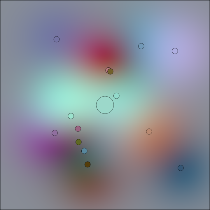
Demonstrates using a two-dimensional Radial Basis Function (RBF) interpolator with the user provided 2D input points, their corresponding values (colors in this demo), a smoothing factor, and a radial basis function kernel.

The program chooses 14 random points in the window area leaving a 100 pixels margin around the borders and assigns a randomized color to each point.

Next it creates the interpolator using those points and colors, a smoothing factor and the RBF function used for interpolation. This function takes a squared distance as input and returns a scalar value representing the influence of points at that distance.

A ShadeStyle implementing the RBF interpolation is created next, used to render the background gradient interpolating all points and their colors.

After rendering the background, the original points and their colors are drawn as circles for reference.

Finally, the current mouse position is used for sampling a color from the interpolator and displayed for comparison. Notice that even if the fill color is flat, it may look like a gradient due to the changing colors in the surrounding pixels.

source code

rbf/RbfInterpolation02

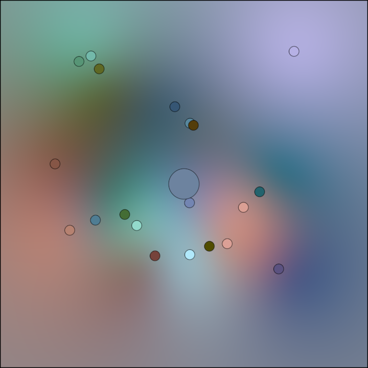
Demonstrates using a two-dimensional Radial Basis Function (RBF) interpolator with the user provided 2D input points, their corresponding values (colors in this demo), a smoothing factor, and a radial basis function kernel.

The program chooses 20 random points in the window area leaving a 100 pixels margin around the borders and assigns a randomized color to each point.

Next it creates the interpolator using those points and colors, a smoothing factor and the RBF function used for interpolation. This function takes a squared distance as input and returns a scalar value representing the influence of points at that distance.

A ShadeStyle implementing the same RBF interpolation is created next, used to render the background gradient interpolating all points and their colors.

After rendering the background, the original points and their colors are drawn as circles for reference.

Finally, the current mouse position is used for sampling a color from the interpolator and displayed for comparison. Notice that even if the fill color is flat, it may look like a gradient due to the changing colors in the surrounding pixels.

source code

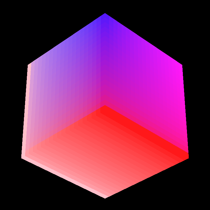
simplexrange/DemoSimplexRange3D01

Demonstrates the use of the SimplexRange3D class. Its constructor takes 4 instances of a LinearType (something that can be interpolated linearly, like ColorRGBa). The SimplexRange3D instance provides a value() method that returns a LinearType interpolated across the 4 constructor arguments using a normalized 3D coordinate.

This demo program creates a 3D grid of 20x20x20 unit 3D cubes. Their color is set by interpolating their XYZ index across the 4 input colors.

2D, 4D and ND varieties are also provided by SimplexRange.

Simplex Range* is not to be confused with Simplex Noise.

source code